Pgvector 0.5.0 Feature Highlights and HOWTOs
It’s here! pgvector 0.5.0 is released and has some incredible new features. pgvector is an open-source project that brings vector database capabilities to PostgreSQL. The pgvector community is moving very rapidly on adding new features, so I thought it prudent to put together some highlights of the 0.5.0 release.
Here’s a quick list of highlights, though I encourage you read the rest in depth and explore on your own!
This is a big release, so let’s dive right in.
New index type: Hierarchical Navigable Small Worlds (hnsw)
The biggest highlight of the pgvector 0.5.0 release is the introduction of the hnsw index type. hnsw is based on the hierarchical navigable small worlds paper, which describes an indexing technique that creates layers of increasingly dense “neighborhoods” of vectors. The main idea of HNSW is that you can achieve a better performance/recall ratio by connecting vectors that are close to each other, so that when you perform similarity search, you have a higher likelihood of finding the exact nearest neighbors you’re looking for.
Beyond performance, pgvector’s HNSW implementation has several notable features:
- “Build as you go”: With HNSW, you can create an index on an empty table and add vectors as you go without impacting recall! This is different from
ivfflat, where you first need to load your vectors before building the index to find optimal centers for better recall. As you add more data to yourivfflatindex, you may also need to re-index to find updated centers. - Update and delete: pgvector’s HNSW implementation lets you update and delete vectors from the index, as part of standard
UPDATEandDELETEqueries. Many HNSW implementations do not support this feature. - Concurrent inserts: Additionally, pgvector’s HNSW implementations lets you concurrently insert values into the index, making it easier to simultaneously load data from multiple sources.
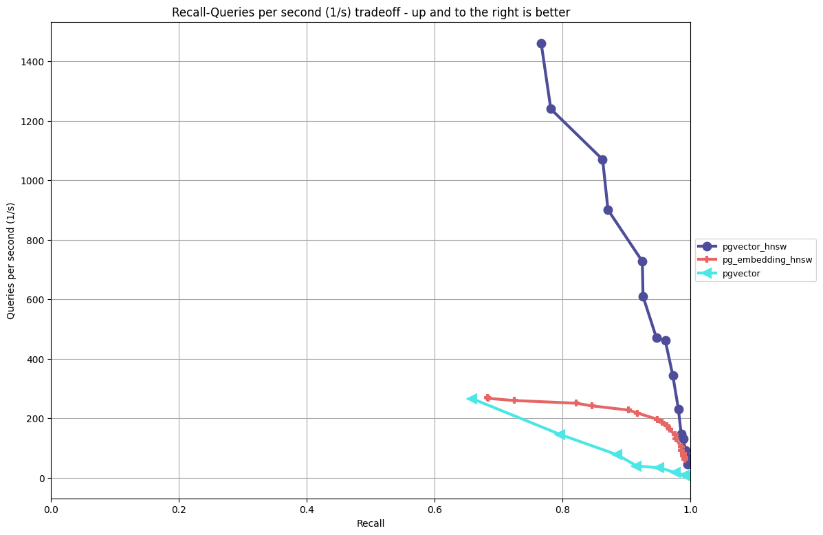
In a previous post, I went into depth on the HNSW performance for pgvector with benchmarks that compared it to ivfflat and pg_embedding’s HNSW implementation. The chart below shows the performance/recall tradeoffs on OpenAI-style embedding data using cosine distance (for full testing methodology and the ANN Benchmark framework. Please read the previous post) for more details on the test methodology and other considerations (index build time, index size on disk):
Instead of focusing on benchmarking in this post, I want to provide guidance on how to use the key parameters in hnsw so you understand the ramifications on your performance/recall ratio and index build times.
In the previous post, we reviewed the 3 parameters that are part of the HNSW algorithm. We’ll break them down to where they are applicable in pgvector’s hnsw implementation:
Index building options
These options are available in the WITH clause of CREATE INDEX, e.g.
CREATE TABLE vecs (id int PRIMARY KEY, embedding vector(768));

CREATE INDEX ON vecs USING hnsw(embedding vector_l2_ops) WITH (m=16, ef_construction=64);
m: (default:16; range:2to100) Indicates how many bidirectional links (or paths) exist between each indexed element. Setting this to a higher number can increase recall, but can also significantly increase index build time and may impact query performance.ef_construction: (default:64; range:4to1000) Indicates how many nearest neighbors to check while adding an element to the index. Increasing this value can increase recall, but will also increase index build time. This value must also be at least doublem, e.g. ifmis24thenef_constructionmust be at least48.
Note that as of this writing, you must specify the operator class to use with the hnsw index. For example, to use cosine distance with an HNSW index, you would use a command similar to the below:
CREATE INDEX ON vecs USING hnsw(embedding vector_cosine_ops);
Index search options
hnsw.ef_search: (default:40; range1to1000) Indicates the number of nearest neighbors to keep in a “dynamic list” while keeping the search. A large value can improve recall, usually with a tradeoff in performance. You needhnsw.ef_searchbe at least as big as yourLIMITvalue.
How to use hnsw in pgvector
The default index build settings are chosen to optimize build time relative to the recall you can achieve during search. If you’re not getting the recall that you expect for your data set, first try increasing the value of ef_construction before adjusting m, as adjusting ef_construction is often a faster operation. There are some studies that show that increasing m can help with recall for higher dimensionality data sets, though in the previous post we saw that pgvector could process OpenAI-style embeddings effectively with high recall.
You can increase performance of your search queries by lowing the value hnsw.ef_search, e.g. set hnsw.ef_search to 20, though note that this could impact your recall:
SET hnsw.ef_search TO 20;
SELECT *
FROM vecs
ORDER BY q <-> embedding
LIMIT 10;
Improved performance of distance functions
Speed is paramount when computing distance between two vectors. Any way you can shave off computation time means you can build indexes and search for vectors more quickly.
pgvector 0.5.0 does exactly this, improving distance calculations across the board with noticeable gains for ARM64 architecture. By default, pgvector can use CPU acceleration for vector processing through compile flags, and writing the implementation code in certain ways can help unlock performance gains once its compiled.
The gains in pgvector 0.5.0 are noticeable. To demonstrate this, I ran an experiment on my Mac M1 Pro (2021 edition, 8 CPI, 16 GB RAM) to show the speedup in building an ivfflat index with both Euclidean (vector_l2_ops, or the default operator class) and cosine distnace (vector_cosine_ops) on a table with 1,000,000 768-dimensional vectors using PLAIN storage:
CREATE TABLE vecs (id int PRIMARY KEY, embedding vector(768));
ALTER TABLE vecs ALTER COLUMN embedding SET STORAGE PLAIN;
Below are some of the relevant local settings used to test the index builds:
shared_buffers:4GBmax_wal_size:10GBwork_mem:8MBmax_parallel_mainetance_workers:0
Before each run, I ensured that the vecs table was loaded into memory using the pg_prewarm extension:
SELECT pg_prewarm('vecs');
Finally, I created the ivfflat index with lists set to 100. Note that this was to run a series of tests quickly; the recommended value of lists for 1,000,000 rows is 1000. The effect of the distance calculations may be more pronounced with a larger value of lists.
Below is a table summarizing the results. Please note that these results are directional, particularly due to the value of lists:
| Version | Euclidean (s) | cosine (s) |
|---|---|---|
| 0.4.4 | 71.66 | 69.92 |
| 0.5.0 | 45.65 | 64.02 |
The above test showed a noticeable improvement with Euclidean distance and a marginal improvement with cosine distance. Andrew Kane’s tests showed a greater speedup across all distance functions on ARM64 systems. That said, you should likely see some performance gains in your pgvector workloads, with these being most pronounced on tasks with many distance computations (e.g. index builds, searches over large sets of vectors).
Parallelization of ivfflat index builds
ivfflat is comparatively fast when it comes to building indexes, though there are always ways to improve performance. One area is adding parallelization to simultaneously perform operations. To understand how parallelism can benefit ivfflat, first let’s explore the different phases of the index build. Recall that we can build an ivfflat index on a table using a query like the one below:
CREATE INDEX ON vecs USING ivfflat(embedding) WITH (lists=100);
Now, let’s look at the different build phases:
- k-means: pgvector samples a subset of all of the vectors in the table to determine
kcenters, wherekis the value oflists. Using the above query, the value ofkis100. - assignment: pgvector then goes through every record in the table and assigns it to its closest lists, where the distance is calculated using the selected distance operator (e.g. Euclidean).
- sort: pgvector then sorts the records in each list
- write-to-disk: Finally, pgvector writes the index to disk.
There are two areas here that can benefit from parallelization:
- k-means: K-means is fairly computational heavy, but it’s also easily parallelizable.
- assignment: During the assignment phase, pgvector must load every record from the table, which can take a long time if the table is very large.
Analysis (to be shown further down) around where pgvector was spending the most time during the index building process showed that pgvector was spending the most time in the assignment phase, particularly as the size of the indexable dataset grew. While the time spent in k-means grew quadratically with the number of lists, it was still only a fraction of the time spent compared to assignment. Interestingly, write-to-disk stayed relative constant as a percentage of time across the tests.
pgvector 0.5.0 added parallelization around the assignment phase, specifically, spawning multiple parallel maintenance workers to scan the table and assign records to the closest list. There are a few parameters you need to be aware of when using this feature:
max_parallel_maintenance_workers: This is the max number of parallel workers PostgreSQL will spawn for a mainetnance operation, such as an index build. This defaults to2, so you may need to set it higher to get the full benefit of this feature.max_parallel_workers: This is the max number of parallel workers PostgreSQL spawns for parallel operations. This defaults to8in PostgreSQL, so you may need to increase it along withmax_parallel_maintenance_workersbased upon how much parallelism you need.min_parallel_table_scan_size: This parameter determines how much data must be scanned to determine when and how many parallel workers to spawn. If you’re usingEXTENDED/ TOAST storage (the default) for your vectors, you may not be getting a parallel scan because PostgreSQL will only consider the amount of space used in the main table, not the TOAST table. Setting this to a lower value (e.g.SET min_parallel_table_scan_size TO 1) may help you spawn more parallel workers.
Below is an example of the impact of parallelization on a 1,000,000 set of 768-dimensional vectors (note, to see parallel workers spawned in your session, you’ll have to run SET client_min_messages TO 'DEBUG1';):
Serial build:
CREATE INDEX ON vecs USING ivfflat(embedding) WITH (lists=500);
DEBUG:  building index "vecs_embedding_idx" on table "vecs" serially
CREATE INDEX
Time: 112836.829 ms (01:52.837)
Parallel build with 2 workers (including the leader, so really “3” workers :):
SET max_parallel_maintenance_workers TO 2;
CREATE INDEX ON vecs USING ivfflat(embedding) WITH (lists=500);
DEBUG:  using 2 parallel workers
DEBUG:  worker processed 331820 tuples
DEBUG:  worker processed 331764 tuples
DEBUG:  leader processed 336416 tuples
CREATE INDEX
Time: 61849.137 ms (01:01.849)
We can see that there is almost a 2x speedup with parallel builds. But how much is too much? Let’s see what happens when we allow for PostgreSQL to use more parallel workers on this data set:
SET max_parallel_maintenance_workers TO 8;
CREATE INDEX ON vecs USING ivfflat(embedding) WITH (lists=500);
DEBUG:  using 6 parallel workers
DEBUG:  worker processed 142740 tuples
DEBUG:  worker processed 142394 tuples
DEBUG:  worker processed 142192 tuples
DEBUG:  worker processed 142316 tuples
DEBUG:  worker processed 142674 tuples
DEBUG:  leader processed 142284 tuples
DEBUG:  worker processed 145400 tuples
CREATE INDEX
Time: 67140.314 ms (01:07.140)
We can see that for this data set, we were able to achieve max performance with only 2 workers, and the leader.
Where does this feature shave off time? Let’s look at a comparison between a few different runs and times between the different phases:
1,000,000 768-dim vectors, lists=1000
Time measured in seconds.
| Build | Total | k-means | assignment | sort | write-to-disk |
|---|---|---|---|---|---|
| Serial | 185 | 32 | 130 | 0.04 | 23 |
| Parallel | 80 | 34 | 21 | 1.3 | 24 |
| Speedup | 2.3x | 6.1x |
In the above experiment, we see that we get a 2x+ overall speedup, with a 6x improvement in the assignment phase, though note that the sort has a significant slowdown (albeit it’s not noticeable). Let’s add more vectors into the mix.
5,000,000 768-dim vectors, lists=2000
Time measured in seconds.
| Build | Total | k-means | assignment | sort | write-to-disk |
|---|---|---|---|---|---|
| Serial | 1724 | 168 | 1430 | 0.04 | 126 |
| Parallel | 551 | 173 | 253 | 4 | 120 |
| Speedup | 3.1x | 5.64x |
Again, in this experiment we see that we save the most time in the assignment phase, though note that the sort time increases roughly linearly as we add more vectors into the build.
Finally, let’s look at one very large example!
100,000,000 384-dim vectors, lists=1000
A few things to note about this test:
- First, you’d normally use a larger value of lists to drive a better performance/recall ratio across your data set.
- I mainly experimented with different values of
max_parallel_maintenance_workers, and for this data set, the optimal value was around32. - Finally, I stopped the tests before the write-to-disk phase completed, but everything was trending much faster than the 23 hours it took to build this serially!
Time is in hours. All builds were in parallel:
| Workers | Total | k-means | assignment | sort |
|---|---|---|---|---|
| 10 | 17.9 | 0.36 | 17.5 | 0.08 |
| 16 | 11.3 | 0.38 | 10.6 | 0.34 |
| 32 | 10.6 | 0.37 | 9.3 | 1.01 |
| 48 | 11.7 | 0.36 | 10.1 | 1.26 |
Overall, if you have larger data sets, you should see improvements in ivfflat build times, particularly for larger data sets.
Other features
pgvector 0.5.0 is a pretty big release, so don’t miss out on these other items:
SUMaggregates: You can now sum up all your vectors, e.g.SELECT sum(embedding) FROM vecs;.- Manhattan / Taxicab / L1 distance: This release adds the
l1_distancefunction so you can find the Manhattan distance between two vectors (which I personally find very helpful). - Element-wise multiplication: You can now multiple two vectors by each other, e.g.
SELECT '[1,2,3]'::vector(3) * '[4,5,6]'::vector(3).
What’s next?
Ready to try out or upgrade to pgvector 0.5.0? If you’re already using pgvector, once you’ve installed the new version into your database, you can upgrade to 0.5.0 using the following command:
ALTER EXTENSION vector UPDATE;
or explicitly via:
ALTER EXTENSION vector UPDATE TO '0.5.0';
There’s still more to come in pgvector. The 0.5.0 release will help support more vector-driven workloads on PostgreSQL, and is a great setup for future releases that will further expand the capabilities of PostgreSQL as a vector database.
And last but not least, but a huge THANK YOU to everyone who’s worked on pgvector to date, whether its coding, testing, providing feedback, and contributing ideas. A very special thanks to Andrew Kane for his tireless work on the 0.5.0 release, and also many thanks to Pavel Borisov who did the work unlocked the performance gains ont he distance operations.
As awesome as the 0.5.0 release of pgvector is, the best has yet to come. Stay tuned!